#TheMoment tweets
On Sunday morning I came across a tweet by NPR’s Lulu Garcia-Navarro morning asking people when they knew things were going to be different due to COVID.
We all have #TheMoment when we knew things were going to be different. Where were you and what were you thinking a year ago? We are one year into this pandemic. Tell us @NPR @NPRWeekend
— Lulu (@lourdesgnavarro) February 28, 2021
Whenever I read replies to a tweet like this I’m always tempted to scrape all the replies and take a look at the data to see if anything interesting emerges. So I go ahead and load the awesome rtweet package and then I remember that the task of getting all replies to a tweet is not super straightforward – there is even an open issue about this on the package repo. I feel like over the years I’ve seen more than one write up about solving this problem, and one that came to mind was Jenny Bryan’s, which you can find here. But this solution uses the twitteR package which predates rtweet and hasn’t been updated for a while. It looked like it should be possible to update the code to use rtweet, but I had limited time on a weekend with family responsibilities, so I decided to take the short cut.
Let’s start by loading all the packages I’ll use for this mini analysis:
library(glue)       # for constructing text strings
library(lubridate)  # for working with dates
library(rtweet)     # for getting Twitter data
library(tidytext)   # for working with text data
library(tidyverse)  # for data wrangling and visualisation
library(viridis)    # for colors
library(wordcloud)  # for making a word cloud
Getting replies to the original tweet, kinda…
First, I took a look at the original tweet. The text of the tweet is stored in the text column of the result – I’ll refer to the text column repeatedly throughout this post.
original_tweet <- lookup_tweets("1365844493434572801")
original_tweet$text
## [1] "We all have #TheMoment when we knew things were going to be different. Where were you and what were you thinking a year ago? We are one year into this pandemic. Tell us @NPR @NPRWeekend"The original tweet mentions two screen names: @NPR and @NPRWeekend.
Then, I picked just one reply to the original tweet and took a look at its text:
reply_tweet <- lookup_tweets("1365864066460377088")
reply_tweet$text
## [1] "@lourdesgnavarro @NPR @NPRWeekend On Friday, March 6th (I believe) I saw a tweet with a video from Harvard where @juliettekayyem was saying we should be prepared for our lives to change...and it scared the shit out of me. Hit Costco in the morning but the sadness took a few weeks to kick in. #TheMoment"It contains the original mentions (@NPR and @NPRWeekend) as well as @lourdesgnavarro since it’s a reply to @lourdesgnavarro.
As a short cut, I decided to define replies roughly as “tweets that mention these three screen names, in that order”. I realize that this might be missing some replies as Twitter allows you to deselect mentions when replying to a tweet. It’s also possible this catches some tweets that are not replies to the original tweet but just happens to have these three mentions, in this order. This is why this section is called “getting replies to the original tweet, kinda” and not “getting all replies to the original tweet”.
I set the number of tweets to download (n) to 18000, which is the maximum allowed, though based on the engagement on the original tweet, I didn’t expect there would be that many replies.
replies_raw <- search_tweets(
  q = "@lourdesgnavarro @NPR @NPRWeekend",
  n = 18000
  )
Note that this code isn’t running in real time, so these are replies as of around 10am GMT on the morning of Monday, 1 March. There are 7572 replies in the result.
Cleaning replies
Based on a bit of interactive investigation of the data, I decided to do some data cleaning before analysing it further.
- Remove original tweet: The original tweet is in
replies_rawas well as retweets of that original tweet. Since I want the replies, I’ll filter those out. - Keep only one of each tweet: Some tweets in
replies_raware retweets of each other, so I’ll usedistinct()to make sure each unique tweet text appears once in the data.- Note that the output from the
search_tweets()call has metadata about the tweets, and one of these pieces of information is whether the tweet is a retweet or not. But I wanted to make sure I omit retweets but not quote tweets (as some people put their reply in a quote tweet), so I took thedistinct()approach. It might be possible to get the same, or perhaps a more accurate, result using features from the tweet metadata. - With my approach, if two people tweet the exact same reply, I’ll lose this, but that seems unlikely.
- Note that the output from the
- Remove words from tweets: Each of these tweets include the mentions
@lourdesgnavarro,@NPRWeekend, and@NPRand many also include#TheMoment. I don’t want these appearing on top of the common words I extract from the tweets, so I’ll remove them (along with their lowercase variants)
replies <- replies_raw %>%
  # remove original tweet
  filter(text != original_tweet$text) %>%
  # keep only one of each tweet
  distinct(text, .keep_all = TRUE) %>%
  # remove words from tweets
  mutate(
    text = str_remove_all(text, "@lourdesgnavarro"),
    text = str_remove_all(text, "@NPRWeekend"),
    text = str_remove_all(text, "@nprweekend"),
    text = str_remove_all(text, "@NPR"),
    text = str_remove_all(text, "@npr"),
    text = str_remove_all(text, "#TheMoment")
  )
Common words
Using the tidytext package, I took a look at the most common words in the replies, excluding any stop words.
words <- replies %>%
  unnest_tokens(word, text, "tweets") %>%
  anti_join(stop_words) %>%
  count(word, sort = TRUE)
words
## # A tibble: 13,121 x 2
## word n
## <chr> <int>
## 1 march 1451
## 2 home 1145
## 3 day 839
## 4 amp 800
## 5 time 603
## 6 week 537
## 7 school 517
## 8 weeks 511
## 9 started 495
## 10 2020 478
## # … with 13,111 more rowsThis result isn’t super interesting, but it looks like for most people their “moment” was in March and I was surprised to see February ranked as low as 25th in the list of common words.
words %>%
  rowid_to_column(var = "rank") %>%
  filter(word == "february")
## # A tibble: 1 x 3
## rank word n
## <int> <chr> <int>
## 1 25 february 283Common bigrams
Next I explored common bigrams, which took a bit more fiddling. I am not aware of a predefined list of stop words for bigrams, so I decided to exclude any bigrams where both words are stop words, e.g. “in the”. I also excluded the bigram “https t.co”, which contains URL fragments.
bigrams <- replies %>%
  unnest_tokens(ngram, text, "ngrams", n = 2) %>%
  count(ngram, sort = TRUE) %>%
  # fiddle with stop words
  separate(ngram, into = c("temp_word1", "temp_word2"), remove = FALSE, sep = " ") %>%
  mutate(
    temp_word1_stop = if_else(temp_word1 %in% stop_words$word, TRUE, FALSE),
    temp_word2_stop = if_else(temp_word2 %in% stop_words$word, TRUE, FALSE),
    temp_stop       = temp_word1_stop + temp_word2_stop
  ) %>%
  filter(temp_stop != 2) %>%
  select(!contains("temp")) %>%
  # exclude URL fragments
  filter(ngram != "https t.co")

bigrams
## # A tibble: 75,521 x 2
## ngram n
## <chr> <int>
## 1 shut down 296
## 2 on march 287
## 3 i remember 220
## 4 year ago 207
## 5 spring break 199
## 6 my husband 176
## 7 next day 166
## 8 from home 165
## 9 the nba 162
## 10 a week 160
## # … with 75,511 more rowsMarch comes up again!
When was #TheMoment?
After the initial exploration of common words and bigrams I decided that interesting feature of these data might be the dates mentioned in the tweets. After interactively filtering for various months in the RStudio data viewer to see what sorts of results I get, I decided to focus on bigrams that include the months December through May. And I used readr::parse_number() to do the heavy lifting of extracting numbers from the bigrams.
themoment <- bigrams %>%
  # filter for certain months
  filter(str_detect(ngram, "december|january|february|march|april|may")) %>%
  # add month and day variables
  mutate(
    month = case_when(
      str_detect(ngram, "december") ~ "December",
      str_detect(ngram, "january")  ~ "January",
      str_detect(ngram, "february") ~ "February",
      str_detect(ngram, "march")    ~ "March",
      str_detect(ngram, "april")    ~ "April",
      str_detect(ngram, "may")      ~ "May"
    ),
    day = parse_number(ngram)
    ) %>%
  # only keep actual dates
  filter(!is.na(day), !is.na(month), day <= 31) %>%
  # calculate number of tweets that mention a certain date
  group_by(month, day) %>%
  summarise(n_total = sum(n), .groups = "drop") %>%
  # construct date variable
  mutate(
    date = if_else(month == "December",
                   glue("{month} {day} 2019"),
                   glue("{month} {day} 2020")),
    date = mdy(date)
    ) %>%
  # arrange results by date
  arrange(date)

themoment
## # A tibble: 90 x 4
## month day n_total date
## <chr> <dbl> <int> <date>
## 1 December 14 1 2019-12-14
## 2 December 28 1 2019-12-28
## 3 December 31 2 2019-12-31
## 4 January 3 1 2020-01-03
## 5 January 6 1 2020-01-06
## 6 January 10 1 2020-01-10
## 7 January 11 1 2020-01-11
## 8 January 16 1 2020-01-16
## 9 January 19 1 2020-01-19
## 10 January 20 3 2020-01-20
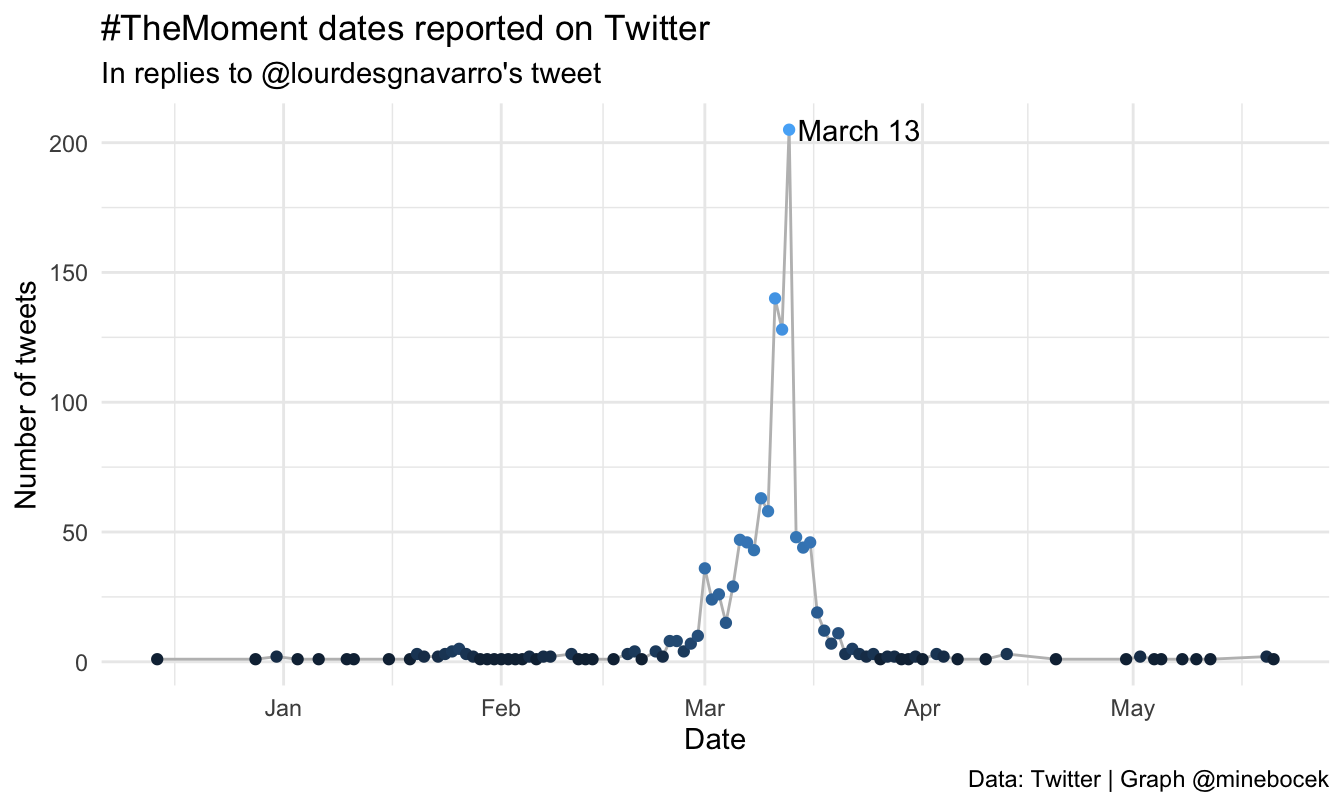
## # … with 80 more rowsLet’s take a look at which dates were most commonly mentioned.
themoment %>%
  arrange(desc(n_total))
## # A tibble: 90 x 4
## month day n_total date
## <chr> <dbl> <int> <date>
## 1 March 13 205 2020-03-13
## 2 March 11 140 2020-03-11
## 3 March 12 128 2020-03-12
## 4 March 9 63 2020-03-09
## 5 March 10 58 2020-03-10
## 6 March 14 48 2020-03-14
## 7 March 6 47 2020-03-06
## 8 March 7 46 2020-03-07
## 9 March 16 46 2020-03-16
## 10 March 15 44 2020-03-15
## # … with 80 more rowsAs expected based on previous results, I see lots of March dates, but March 13 seems to really stand out.
Let’s also visualise these data over time.
ggplot(themoment, aes(x = date, y = n_total)) +
  geom_line(color = "gray") +
  geom_point(aes(color = log(n_total)), show.legend = FALSE) +
  labs(
    x = "Date",
    y = "Number of tweets",
    title = "#TheMoment dates reported on Twitter",
    subtitle = "In replies to @lourdesgnavarro's tweet",
    caption = "Data: Twitter | Graph @minebocek"
  ) +
  annotate(
    "text",
    x = mdy("March 13 2020") + 10,
    y = 205,
    label = "March 13"
  ) +
  theme_minimal()
What happened on March 13, 2020?
I’d like to first acknowledge that March 13, 2020 is an incredibly sad day in history, the day Breonna Taylor was fatally shot in her apartment. I encourage you to read the powerful statement by Black Lives Matter Global Network Foundation in response to Grand Jury verdict in the Breonna Taylor case.
I wanted to see why this date stood out in the replies. This is an opportunity to fix a simplifying assumption I made earlier as well. Some dates are spelled out as “March 13” or “13 March” in the tweets, but some are written as “3/13” or “3-13” or “Mar 13” and various versions of these.
march_13_text <- c(
  "march 13", "13 march",
  "3/13", "3-13",
  "mar 13", "13 mar"
)
march_13_regex <- glue_collapse(march_13_text, sep = "|")
I can now go back to the tweets and filter them for any of these text strings to get all mentions of this date.
march_13_tweets <- replies %>%
  mutate(text = str_to_lower(text)) %>%
  filter(str_detect(text, march_13_regex))
There are 295 such tweets, which is more than what’s shown in the earlier visualisation.
To get a sense of what’s in these tweets, I can again take a look at common words in them. But first, I’ll remove the text strings I searched for, since they will obviously be very common.
march_13_words <- march_13_tweets %>%
  mutate(text = str_remove_all(text, march_13_regex)) %>%
  unnest_tokens(word, text) %>%
  anti_join(stop_words)
## Joining, by = "word"march_13_words %>%
count(word, sort = TRUE)## # A tibble: 1,917 x 2
## word n
## <chr> <int>
## 1 home 102
## 2 school 89
## 3 day 82
## 4 3 73
## 5 2020 54
## 6 friday 54
## 7 weeks 50
## 8 march 44
## 9 amp 40
## 10 closed 39
## # … with 1,907 more rowsIt’s not straightforward to get anything meaningful from this output. I think the “3” comes from mentioning other dates in March (e.g. “3/12”), “2020” is the year and doesn’t tell us anything additional in this context, and “amp” is “&” when tokenized. So I’ll remove these.
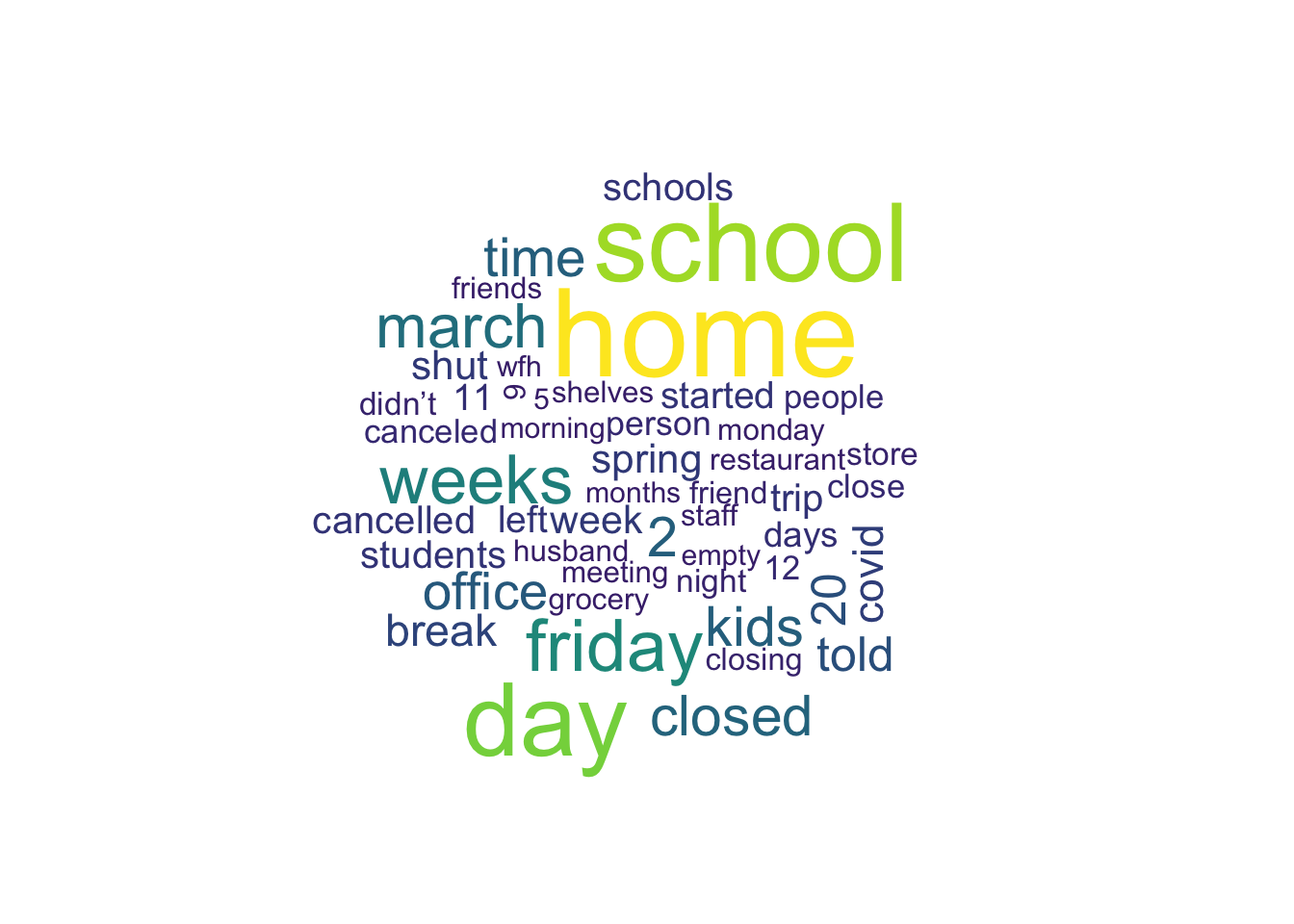
I’m not a huge fan of wordclouds but I think it might be a helpful visualisation here, so I’ll give that a try.
march_13_words %>%
  count(word) %>%
  filter(!(word %in% c("3", "2020", "amp", "https", "t.co"))) %>%
  with(wordcloud(word, n, max.words = 50, colors = viridis::viridis(n = 50)))
Tom Hanks, the NBA, and spring break
As I was perusing the data throughout this analysis, mentions of Tom Hanks and NBA seemed quite frequent. This was surprising to be since the NBA is rarely on my radar (and less so now that I’m in the UK) and I was not expecting the Tom Hanks celebrity effect! Another phrase that stood out was spring break, which is not too unexpected.
Let’s take a look at how many tweets mention these, out of the 5969 total.
replies %>%
  transmute(
    text         = str_to_lower(text),
    tom_hanks    = str_detect(text, "\\btom hanks\\b"),
    nba          = str_detect(text, "\\bnba\\b"),
    spring_break = str_detect(text, "\\bspring break\\b")
    ) %>%
  summarise(
    across(tom_hanks:spring_break, sum)
    ) %>%
  mutate(
    across(tom_hanks:spring_break, ~ . / nrow(replies), .names = "p_{.col}")
    )
## # A tibble: 1 x 6
## tom_hanks nba spring_break p_tom_hanks p_nba p_spring_break
## <int> <int> <int> <dbl> <dbl> <dbl>
## 1 67 218 190 0.0112 0.0365 0.0318Only about 1% of tweets for Tom Hanks and roughly 3% of tweets for NBA and spring break. Not too many actually, but still more than I expected, especially for Tom Hanks.
Conclusion
Perhaps the most unexpected thing about the results of this analysis is how clearly March 13 stands out as a date people mentioned. The other surprising result was people mentioning dates as late as end of May!
There are certainly some holes in this analysis. Text strings I used (both for capturing replies to the original tweet and for including/excluding tweets from the analysis) as well as my regular expressions could be more robust. Additionally, relying on readr::parse_number() solely to get dates is likely not bullet proof.

