Exploring the gt package with the useR 2019 schedule
I have been meaning to try out the gt package for a while now, but didn’t really have a great use case for it. However over the last few days I have been looking over the useR 2019 schedule and felt like I would have an easier time picking talks yo attend if the schedule was formatted in wide format (talks occurring at the same time in different rooms listed next to each other) as opposed to the long format.1
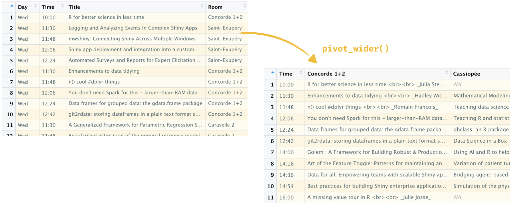
Since “wide” and “long” are not well-defined concepts, let me first clarify what I mean by them in this context: wide refers to data frames where each row is a time slot and long refers to data frames where each row is a talk.
I have to admit some of the data processing steps I’ve implemented for achieving the look I wanted are more manual than I would have liked, but overall I’m pretty happy with the result! You can view and interact with the resulting flexdashboard here.2 And the code associated with this mini-project can be found here.
Some highlights are:
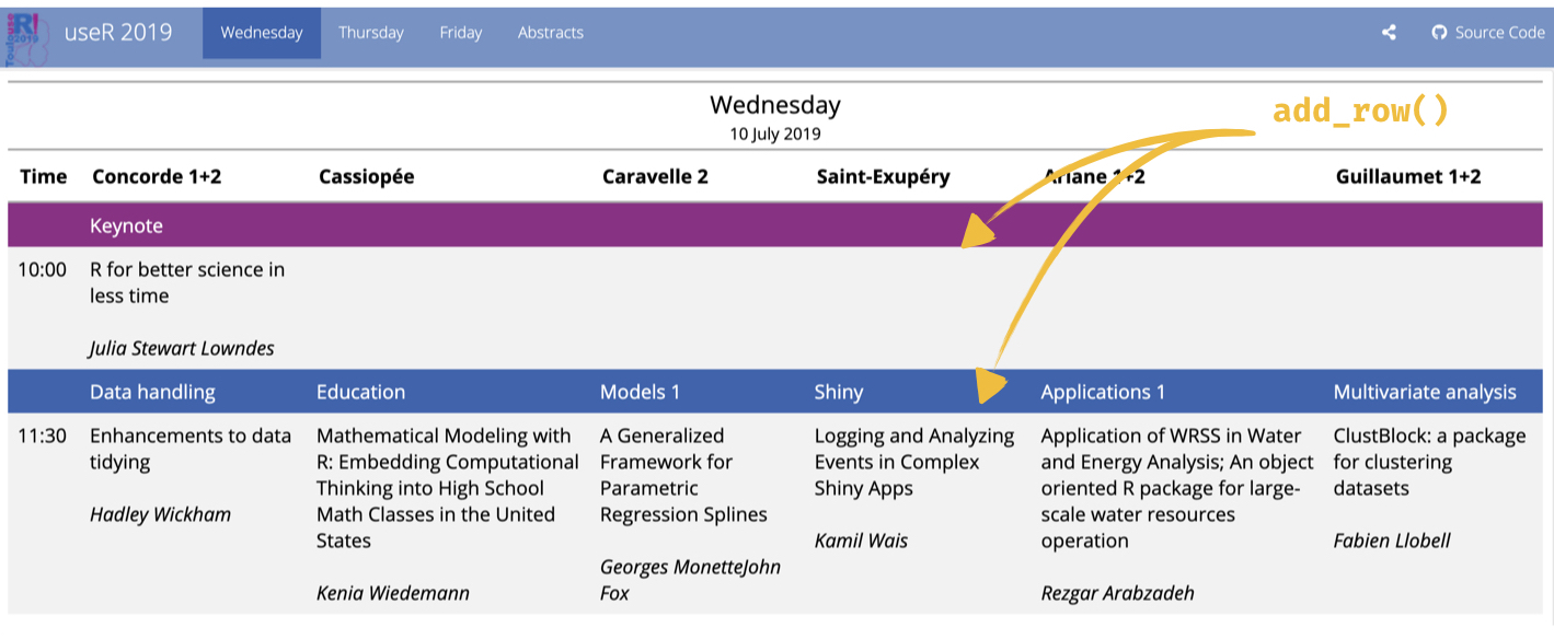
- I feel like I rarely have a use for
tibble::add_row(), but this function came really handy for this task when adding what one might call “interim column headers” (session names). Something that makes sense, but I hadn’t really thought about before, is that when adding multiple rows throughout a data frame the row index changes as you add rows. My tables were pretty short so I counted up where these rows needed to be added, but a more programmatic way to determine the row index would be preferable.
tidyr::pivot_*()functions are da bomb! Going from long to wide format was a breeze withpivot_wider().
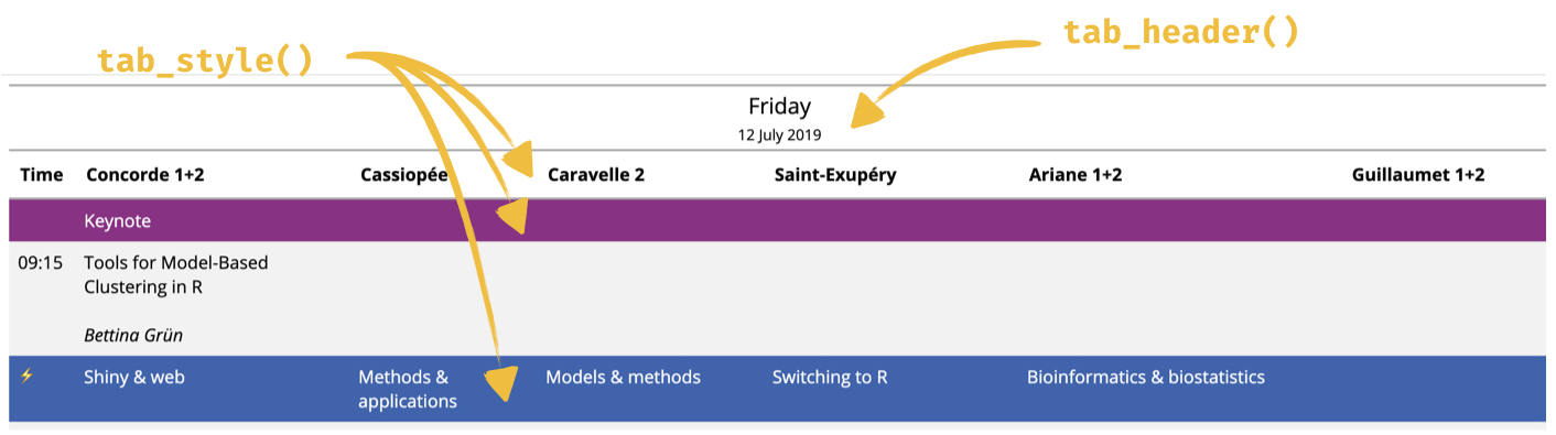
- The gt package has super sleek functionality for styling rows/columns/cells,
and fantastic documentation and website. I did much of this work on a plane without WiFi3 and the figures in the R help files were super helpful for figuring out how the functions work. Every package with some visual aspect to its output should include rendered figures in its help files.
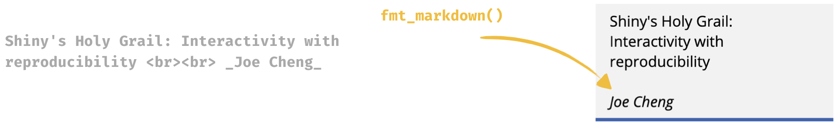
gt::fmt_markdown()is pretty handy for styling text inside cells. You can have a source file that includes markdown formatting in the text, e.g. a spreadsheet with cells with text_italicized_and with this function, the markdown formatting gets reflected in the resulting table.
- Finally, I loved my first foray into gt, but I’m not over my love for
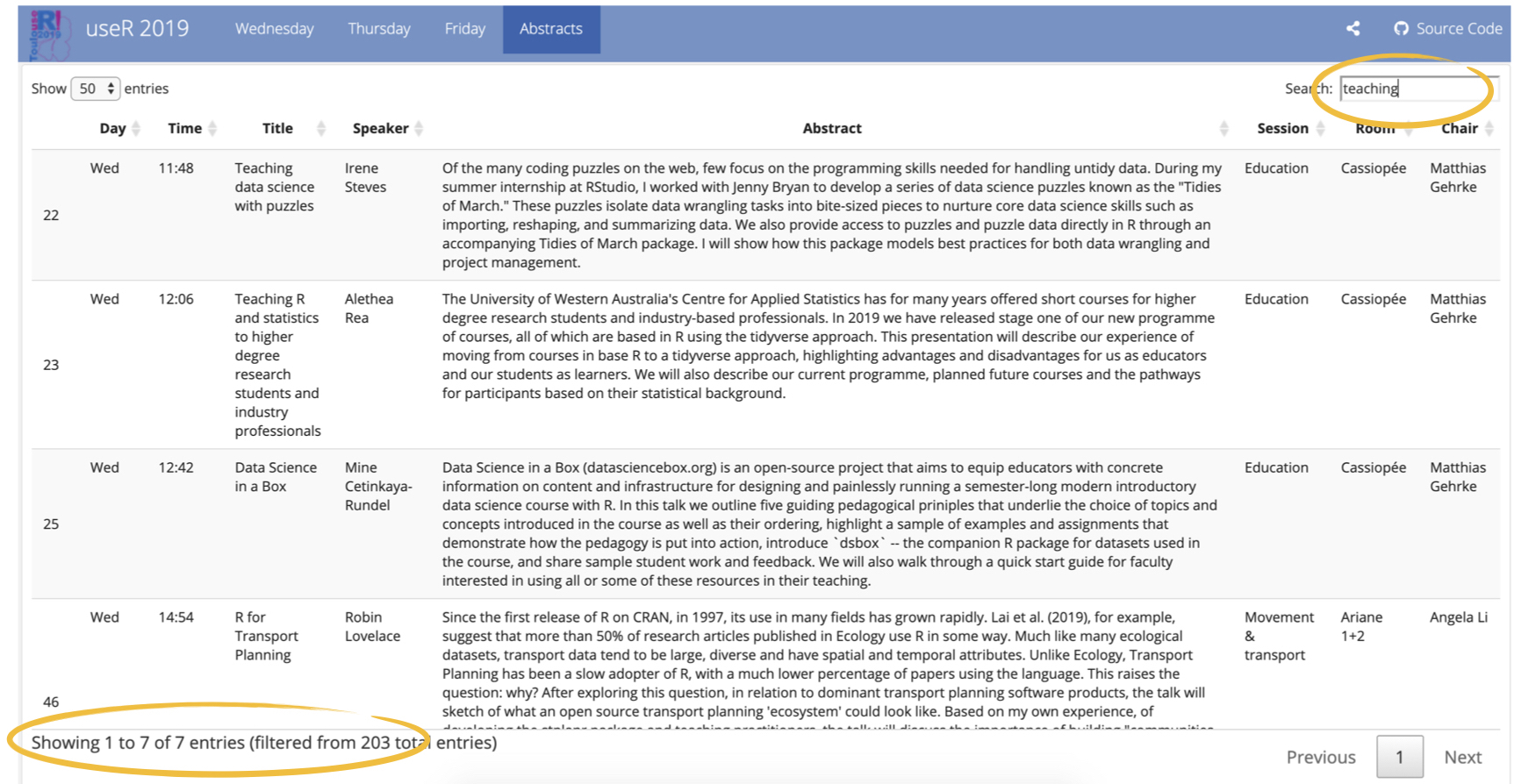
DT::datatable()yet. I was going to build a Shiny app for the abstracts page for searching for keywords, but then I rememberedDT::datatable()has built-in search functionality so I went with that. I much prefer gt for it’s simplicity in building by layers with the pipe operator and its styling, but the out of the box (limited but sufficient) interactivityDT::datatable()offers out of the box is hard to beat
I’m happy to answer any questions about this process. Just don’t ask me whether my conference talk is ready!
Below is a more detailed account of the data scraping, processing, and communication parts of this mini-project.
Scrape
First, I checked that I’m indeed allowed to scrape the useR 2019 website using
robotstxt::paths_allowed():
library(robotstxt)
paths_allowed("http://www.user2019.fr/talk_schedule/")
##
www.user2019.fr## [1] TRUEI used the tidyverse, rvest, glue, and tools packages to scrape and process the data into a format I wanted.
library(tidyverse)
library(rvest)
library(glue)
library(tools)
Data scraping took only two functions, read_html() and html_table():
# read schedule page -----------------------------------------------------------
page <- read_html("http://www.user2019.fr/talk_schedule/")

# extract table ----------------------------------------------------------------
tabs <- page %>%
  html_table("td", header = TRUE)
This results in a list with three elements, one for each day of the conference4: Wednesday, Thursday, and Friday.
Process
Since the format of the tables for each day is essentially the same, I wrote a function to process each one and write out two CSV files per day: one in wide format for the talks and the other in long format for the abstracts.
# function to process data -----------------------------------------------------
process_schedule <- function(day_tab, day_name){

  # remove unused columns ----
  raw <- day_tab %>% select(-2, -Slides)

  # create talks_long ----
  talks_long <- raw %>%
    slice(seq(1, nrow(raw), by = 2)) %>%
    mutate(info = as.character(glue("{Title} <br><br> _{Speaker}_")))

  # create talks_wide ----
  talks_wide <- talks_long %>%
    select(Time, Room, info) %>%
    pivot_wider(names_from = Room, values_from = info) %>%
    select(Time, `Concorde 1+2`, `Cassiopée`, `Caravelle 2`,
           `Saint-Exupéry`, `Ariane 1+2`, `Guillaumet 1+2`)

  # create abstracts_long ----
  abstracts_long <- raw %>%
    slice(seq(2, nrow(raw), by = 2)) %>%
    rename(Abstract = Time) %>%
    select(Abstract) %>%
    bind_cols(talks_long, .) %>%
    mutate(Day = toTitleCase(day_name)) %>%
    select(Day, Time, Title, Speaker, Abstract, Session, Room, Chair)

  # write out ----
  write_csv(talks_wide, glue("data/{day_name}_talks_wide.csv"))
  write_csv(abstracts_long, glue("data/{day_name}_abstracts_long.csv"))

}
Two comments about this function:
- In the scraped data talks appear in the odd numbered rows and the abstracts
appear in the even numbered rows. Hence I used
slice(seq(1, nrow(raw), by = 2))orslice(seq(2, nrow(raw), by = 2))to grab these rows. - You need to have a
data/folder in your working directory for this function to work.
I should admit that I can’t believe this code works with all the accents…
Then I ran the function once per each day. I could have done a map or apply step here, but writing this out three times didn’t seem too cumbersome:
# process days -----------------------------------------------------------------
process_schedule(tabs[[1]], "wed")
process_schedule(tabs[[2]], "thu")
process_schedule(tabs[[3]], "fri")
Communicate
Finally, I used a flexdashboard to put everything together. The code for the flexdashboard can be found here.
A styling note on the dashboard: I used the yeti theme with a custom color navbar (a lighter tint of the blue used for highlighting certain rows).
